
A Glimpse of My Research in Multi-Agent Belief Change
The basic idea behind multi-agent belief change is as follows: We have a network of agents, each of which has some initial beliefs about the state of the world, expressed as formulas of propositional logic. The agents communicate with one another and share their beliefs. Our goal is to determine what each agent will believe after learning as much as possible from other agents connected to it. This process is illustrated below:
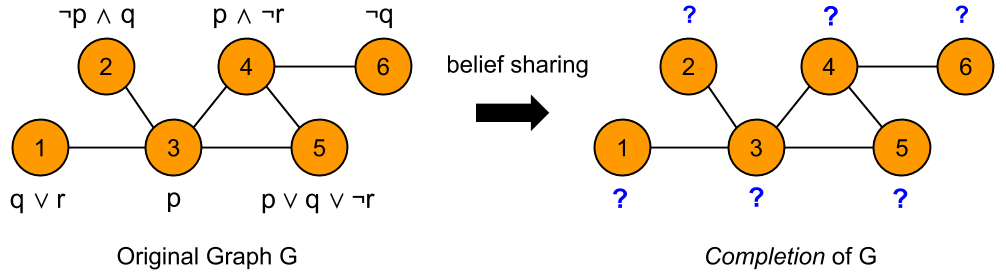
Essentially, we want to find out what formulas are represented by the question marks above. There are many different ways in which beliefs can be shared among agents, and these can be divided into global approaches that update the beliefs of all agents in the graph in a single “one-shot” operation, and iterative approaches that update the beliefs of each agent via a series of local operations. In this post, I’ll focus on two specific iterative approaches, and I’ll present a counterexample that shows that these two approaches are not equivalent.
Preliminary Definitions
We work with an undirected graph $G = \langle V, E \rangle$ where the vertices are identified by an initial sequence of natural numbers, e.g. for $|V| = n$, we have $V = { 1, \dots, n }$. By convention, we denote edges by ordered pairs $(v,w)$ rather than sets ${ v, w }$.
An interpretation of $\mathcal{L}$ is an assignment of truth values to the atoms in $\mathcal{P}$. We represent an interpretation by the set of atoms that are true in the interpretation; the falsity of an atom is indicated by its absence from the set. For example, given $\mathcal{P} = { p, q, r }$, the interpretation where $p$ is false but $q$ and $r$ are true is expressed by the set ${ q, r }$. The set of all interpretations of $\mathcal{L}$ is denoted by $\Omega$. Given a formula $\alpha \in \mathcal{L}$ and an interpretation $M \in \Omega$, we write $M \models \alpha$ only if $M$ makes $\alpha$ true, so that $M$ is a model of $\alpha$. We denote the set of models of $\alpha$ by $Mod(\alpha)$.
Definition (G-Scenario) Given a graph $G = \langle V, E \rangle$, a $G$-scenario is a function $\sigma : V \to \mathcal{L}$ that associates a formula with each vertex $v \in V$.
Definition (G-Interpretation) Given a graph $G = \langle V, E \rangle$, a $G$-interpretation is a function $m : V \to \Omega$ that associates an interpretation with each vertex $v \in V$.
Definition (G-Model) Given a graph $G$ and a $G$-scenario $\sigma$, a $G$-model is a $G$-interpretation $m$ such that $m(v) \models \sigma(v)$.
Let $Mod(\sigma)$ denote the set of all G-models of $\sigma$.
Defining the Model Lifting of a Graph
Here we define a new representation for a graph with propositional formulas at each node, to make explicit the process by which information is shared among agents.
The basic idea is that a vertex $v$ with formula $\sigma(v) = \varphi$ is replaced by a set of vertices representing the models of $\varphi$. For each edge $(v_1,v_2) \in E$, the vertices representing the models of $\sigma(v_1)$ and those representing the models of $\sigma(v_2)$ are connected in a complete bipartite graph. Each edge of the complete bipartite graph is given a label representing the level of disagreement between the models it connects. The completion of a scenario is found by selecting one or more models corresponding at each original vertex such that the labels of the edges involved form inclusion-minimal sets.
For example, given the base graph:
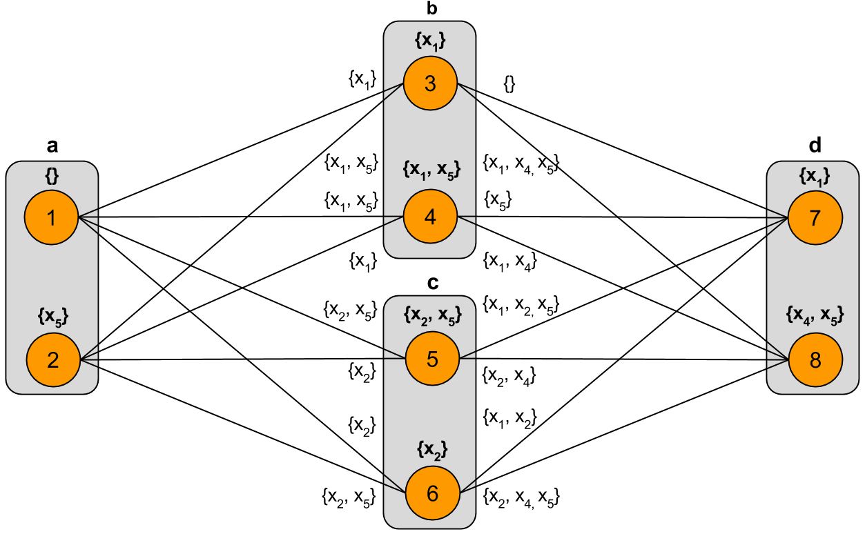
The model lifting corresponding to this base graph is as follows:
Next, I formally define the model lifting of a base graph. Let
\[\text{LiftedVerts}(v) = \{ (v,m) \mid m \in Mod(\sigma(v)) \}\]and let
\[\begin{aligned} \text{LiftedEdges}(v,w) &= \text{LiftedVerts}(v) \times \text{LiftedVerts}(w) \\ &= \{ \langle (v,s), (w,t) \rangle \mid (v,s) \in \text{LiftedVerts}(v), (w,t) \in \text{LiftedVerts}(w) \} \end{aligned}\]For $\langle (v,s), (w,t) \rangle \in \text{LiftedEdges}(v,w)$, we have
\[\text{label}(\langle (v,s), (w,t) \rangle) = \langle (v,w), s \Delta t \rangle\]and
\[\text{label_set}(\langle (v,s), (w,t) \rangle) = s \Delta t\]where $s \Delta t$ represents the symmetric difference between sets $s$ and $t$.
Note: We can have $s, s’, t, t’$ such that $s \neq s’$ and $t \neq t’$ but $s \Delta t = s’ \Delta t’$.
We have a function $\text{sel} : P(\text{LiftedVerts}(v)) \to \text{LiftedVerts}(v)$ that selects exactly one model from the lifted vertex set $\text{LiftedVerts(v)}$ for each $v \in V$.
A model selection is a set of vertices $(v,m)$ with one vertex taken from each set of lifted vertices above a vertex in the base graph. So, a model selection is $\rho = { \text{sel}(\text{LiftedVerts}(v)) \mid v \in V }$.
The change set for an edge $(v,w) \in E$ under selection $\text{sel}$ is:
\[\Delta_{\text{sel}}(v,w) = \text{label}(\text{sel}(\text{LiftedVerts}(v)), \text{sel}(\text{LiftedVerts}(w)))\]So the entire change set for selection $\text{sel}$ is:
\[\Delta(\text{sel}) = \{ \Delta_{\text{sel}}(v,w) \mid (v,w) \in E \}\]Now we define the preference relation over selections based on minimal change sets. For $\text{sel}, \text{sel}’$, we have $\text{sel} \succeq \text{sel}’$ iff $\Delta(\text{sel}) \subseteq \Delta(\text{sel}’)$ and $\text{sel} \succ \text{sel}’$ iff $\Delta(\text{sel}) \subset \Delta(\text{sel}’)$.
We can also define the set of all possible change sets for an edge $(v,w)$ as follows:
\[\Delta(v,w) = \{ \text{label}(\langle (v,s), (w,t) \rangle) \mid (v,s) \in \text{LiftedVerts}(v) \text{ and } (w,t) \in \text{LiftedVerts}(w) \}\]alternatively,
\[\Delta(v,w) = \{ \text{label}(\text{sel}(\text{LiftedVerts}(v)), \text{sel}(\text{LiftedVerts}(w))) \mid \text{sel} \in S \}\]where $S$ is the set of all possible selection functions.
$\Delta(v,w)$ is a partially-ordered set, and thus has minimal elements. Let the inclusion-minimal elements of $\Delta(v,w)$ be denoted $Min(\Delta(v,w), \subseteq)$.
We can use this to define preferred lifted edges to be those lifted edges that are labelled by minimal change set elements. Importantly, there may be several lifted edges labelled by the same minimal change set elements.
For two edges $e, e’ \in \text{LiftedEdges}(v,w)$, define $e \succeq e’$ iff $\text{label_set}(e) \subseteq \text{label_set}(e’)$ and $e \succ e’$ iff $\text{label_set}(e) \subset \text{label_set}(e’)$.
Let the set of preferred lifted edges above base edge $(v,w)$ be $Pref(\text{LiftedEdges}(v,w), \succeq)$. This is the set of lifted edges with minimal labels above $(v,w)$.
Two Forms of Iterated Belief Change
There are (at least) two different forms of iteration that can be defined in this framework. In the first form of iteration, called simple iteration, each agent repeatedly updates its beliefs by taking into account the beliefs of its immediate neighbors. In the second form of iteration, called expanding iteration, an agent first updates its beliefs by taking into account the beliefs of its immediate neighbors, and then further updates its beliefs by taking into account the beliefs of neighbors at distance $\leq 2$, and then neighbors at distance $\leq 3$, and so on. This process ends when the expanding neighborhood about an agent reaches the periphery of the graph, so that the beliefs of all agents in the graph are taken into account. It is important to note that each agent performs this expanding iteration in parallel, and while an agent is considering larger and larger neighborhoods, the graph is stationary; that is, the beliefs of the agents throughout the graph stay fixed while the expansion takes place. Only after a node has updated its beliefs with respect to all neighborhoods up until the end of the graph are its “publicly visible” beliefs updated.
There are several questions that can be asked about these forms of iteration, the primary one being whether they yield equivalent results or not.
Proving that the Forms of Iteration are Not Equivalent
Recently, in my research, I found a counterexample to the statement that expanding iteration is equivalent to simple iteration (equivalence in the sense that the same models are selected at each vertex in the fixpoints reached by the different approaches.)
The rest of this post presents this counterexample in detail, showing what happens in each step of expanding iteration and in each step of simple iteration.
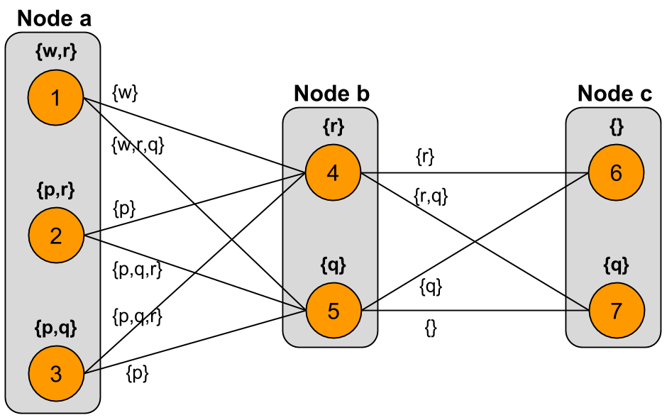
We start with the following model lifting:
I will show that the models selected at node $a$ in the fixpoint of expanding iteration from $a$ differ from the models selected at $a$ in the fixpoint of simple iteration (wherein each vertex repeatedly takes into account the models of its immediate neighbors).
Expanding Iteration From Node $a$
For the first level of expansion centered at node $a$, we consider the following graph:
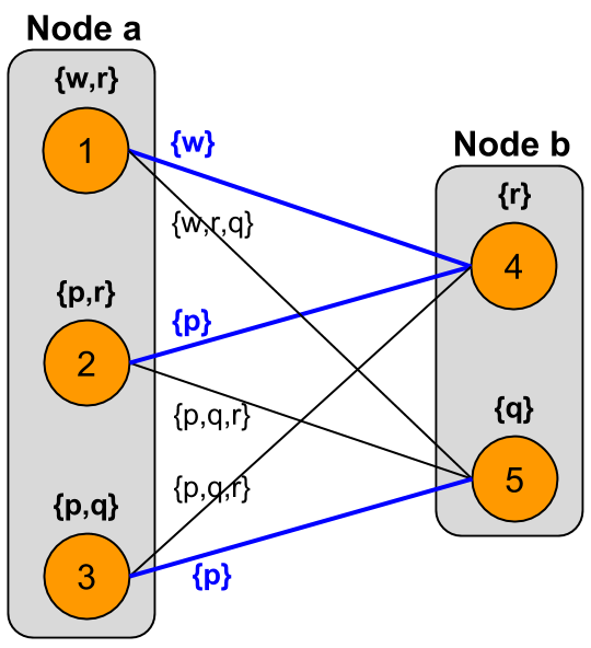
The preferred lifted edges are highlighted in blue; these are the edges labelled by inclusion-minimal sets of atoms. Note that there is a unique lifted edge with the minimal label $\{ w \}$, while there are two different lifted edges with the minimal label $\{ p \}$.
The table below shows the change set elements induced by lifted edges involved in each possible model selection:
| Model Selection | $(a, b)$ |
|---|---|
| 1, 4 | $\{ w \}$ |
| 1, 5 | $\{ w, r, q \}$ |
| 2, 4 | $\{ p \}$ |
| 2, 5 | $\{ p, q, r \}$ |
| 3, 4 | $\{ p, q, r \}$ |
| 3, 5 | $\{ p \}$ |
We find that model selections $\{ 1, 4 \}$, $\{ 2, 4 \}$, and $\{ 3, 5 \}$ yield inclusion-minimal change sets. Thus, each of the models $1$, $2$, and $3$ is involved in at least one minimal change set, and so each is selected at node $a$.
Therefore, in the first level of expansion about node $a$, we select all of the original models at $a$ – no model is dropped, and all of $a$’s original models are available to be selected in the second level of expansion.
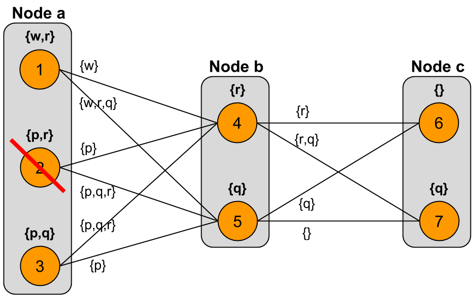
For the second level of expansion centered at node $a$, we consider the following graph:

Now we look at the change sets associated with every possible selection of models in this level-2 graph:
| Model Selection | $(a, b)$ | $(b, c)$ |
|---|---|---|
| 1, 4, 6 | $\{ w \}$ | $\{ r \}$ |
| 1, 4, 7 | $\{ w \}$ | $\{ r, q \}$ |
| 1, 5, 6 | $\{ w, r, q \}$ | $\{ q \}$ |
| 1, 5, 7 | $\{ w, r, q \}$ | $\{ \}$ |
| 2, 4, 6 | $\{ p \}$ | $\{ r \}$ |
| 2, 4, 7 | $\{ p \}$ | $\{ r, q \}$ |
| 2, 5, 6 | $\{ p, q, r \}$ | $\{ q \}$ |
| 2, 5, 7 | $\{ p, q, r \}$ | $\{ \}$ |
| 3, 4, 6 | $\{ p, q, r \}$ | $\{ r \}$ |
| 3, 4, 7 | $\{ p, q, r \}$ | $\{ r, q \}$ |
| 3, 5, 6 | $\{ p \}$ | $\{ q \}$ |
| 3, 5, 7 | $\{ p \}$ | $\{ \}$ |
We see that only the model selections $\{ 1, 4, 6 \}$, $\{ 1, 5, 7 \}$, and $\{ 3, 5, 7 \}$ yield inclusion-minimal change sets. Models $1$ and $3$ are involved in minimal change sets, and are thus selected at the second level of expansion. Note that model $2$ is not involved in any minimal change set; therefore, model $2$ will be dropped at this level of expansion.
The second level of expansion is also the last level, since we have reached the periphery of the graph. Crucially, at the second level of expansion, model $2$ was dropped from the set of models at $a$. The result of expanding iteration about node $a$ is shown in the graph below. Note that in this graph, we do not show the results of expanding iteration about the nodes $b$ and $c$ (which would be done in parallel with expansion about $a$); only the models of $a$ are updated here:
Simple Iteration
Next we look at the results obtained at the fixpoint of simple iteration in this graph. By simple iteration, we mean fixed-radius iteration with radius 1, so that each node repeatedly updates its models by taking into account the models of its immediate neighbors.
Iteration 1, Node $a$
For the first simple iteration about node $a$, we consider the graph:
The change sets associated with each possible model selection are shown below:
| Model Selection | $(a, b)$ |
|---|---|
| 1, 4 | $\{ w \}$ |
| 1, 5 | $\{ w, r, q \}$ |
| 2, 4 | $\{ p \}$ |
| 2, 5 | $\{ p, q, r \}$ |
| 3, 4 | $\{ p, q, r \}$ |
| 3, 5 | $\{ p \}$ |
Since models $1$, $2$, and $3$ from node $a$ are each involved in at least one minimal change set, they are all selected in the first simple iteration.
Iteration 1, Node $b$
For the first simple iteration about node $b$, we consider the graph:
The change sets associated with each possible model selection are shown below:
| Model Selection | $(a, b)$ | $(b, c)$ |
|---|---|---|
| 1, 4, 6 | $\{ w \}$ | $\{ r \}$ |
| 1, 4, 7 | $\{ w \}$ | $\{ r, q \}$ |
| 1, 5, 6 | $\{ w, r, q \}$ | $\{ q \}$ |
| 1, 5, 7 | $\{ w, r, q \}$ | $\{ \}$ |
| 2, 4, 6 | $\{ p \}$ | $\{ r \}$ |
| 2, 4, 7 | $\{ p \}$ | $\{ r, q \}$ |
| 2, 5, 6 | $\{ p, q, r \}$ | $\{ q \}$ |
| 2, 5, 7 | $\{ p, q, r \}$ | $\{ \}$ |
| 3, 4, 6 | $\{ p, q, r \}$ | $\{ r \}$ |
| 3, 4, 7 | $\{ p, q, r \}$ | $\{ r, q \}$ |
| 3, 5, 6 | $\{ p \}$ | $\{ q \}$ |
| 3, 5, 7 | $\{ p \}$ | $\{ \}$ |
We find that model selections $\{ 1, 4, 6 \}$, $\{ 1, 5, 7 \}$, and $\{ 3, 5, 7 \}$ yield inclusion-minimal change sets. Thus, we see that both models $4$ and $5$ from node $b$ are involved in at least one minimal change set, and so both are selected at $b$ in the first simple iteration.
Iteration 1, Node $c$
For the first simple iteration about node $c$, we consider the graph:
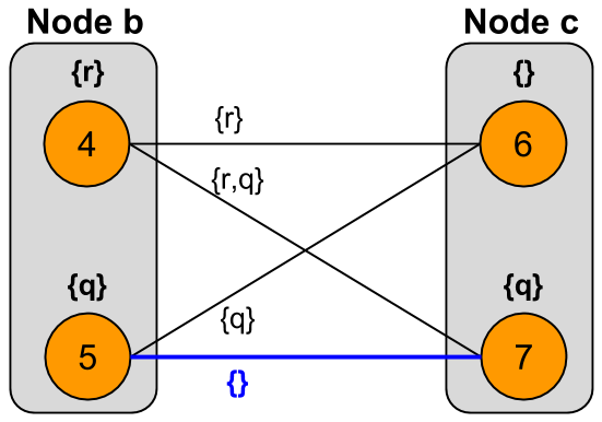
The change sets associated with each possible model selection are shown below:
| Model Selection | $(b, c)$ |
|---|---|
| 4, 6 | $\{ r \}$ |
| 4, 7 | $\{ q, r \}$ |
| 5, 6 | $\{ q \}$ |
| 5, 7 | $\{ \}$ |
Here, we see that there is only one model selection, $\{ 5, 7 \}$, that yields a minimal change set. Thus, only model $7$ from node $c$ is selected in the first simple iteration; model $6$ is dropped.
The Graph After One Complete Simple Iteration
The only change that took place following the first simple iteration was that model $6$ was dropped from node $c$. The graph after one complete simple iteration is as follows:
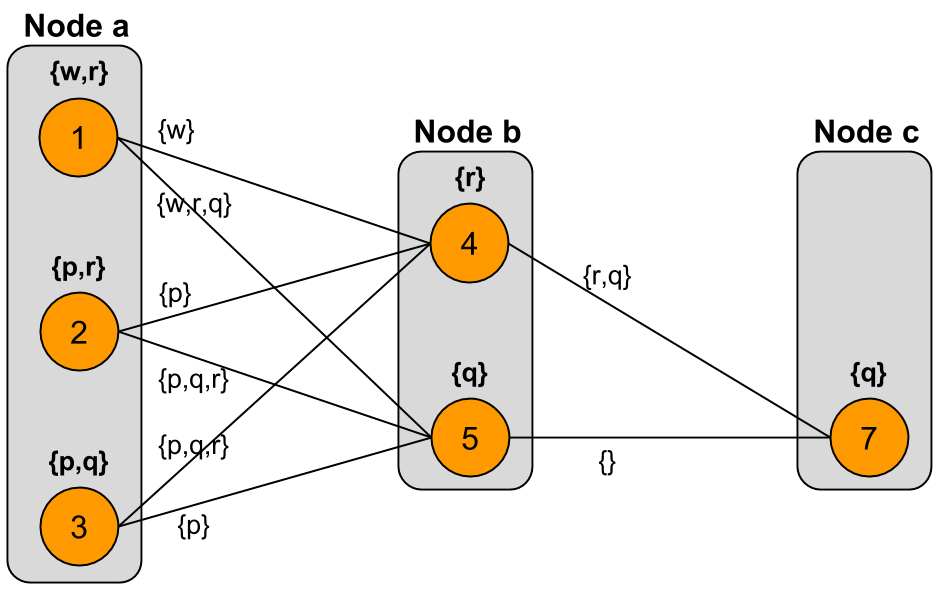
In considering what will happen in the second simple iteration, we note that the models at $b$ have not changed since the start, and since $b$ is the only neighbor of $a$, the second iteration will produce the same results at node $a$ as the first iteration.
That is, the models at node $a$ will not change in iteration 2, because nothing has changed at its only neighbor. Also, we note that nothing can change at node $c$, because $c$ cannot have less than one model. So, in iteration 2 we focus only on node $b$.
Iteration 2, Node $b$
The change sets associated with each possible model selection in the second simple iteration are as follows:
| Model Selection | $(a, b)$ | $(b, c)$ |
|---|---|---|
| 1, 4, 7 | $\{ w \}$ | $\{ q, r \}$ |
| 1, 5, 7 | $\{ w, r, q \}$ | $\{ \}$ |
| 2, 4, 7 | $\{ p \}$ | $\{ q, r \}$ |
| 2, 5, 7 | $\{ p, q, r \}$ | $\{ \}$ |
| 3, 4, 7 | $\{ p, q, r \}$ | $\{ q, r \}$ |
| 3, 5, 7 | $\{ p \}$ | $\{ \}$ |
Here, model selections $\{ 1, 4, 7 \}$, $\{ 1, 5, 7 \}$, and $\{ 3, 5, 7 \}$ yield inclusion-minimal change sets. So, both models $4$ and $5$ are selected at node $b$ in the second simple iteration. Thus, the models at $b$ do not change in the second iteration, and since $b$ is the only neighbor of $a$, this implies that the models at node $a$ will not change anymore in future iterations.
Therefore, the graph reached after one complete simple iteration is the stable state.
We note that in the stable state reached by simple iteration, node $a$ has all of its original models, $1$, $2$, and $3$, while in the stable state reached by expanding iteration about $a$, node $a$ has only models $1$ and $3$.
Thus, expanding iteration and simple (fixed-radius) iteration are not equivalent.